Intermittent Demand Forecast for Spare Parts
Overview
Model a spare part whose weekly history contains more zeros than demand events. This template preserves sparse zero-demand periods instead of filtering them out, compares classic Croston, Syntetos-Boylan Approximation (SBA) Croston, and a trailing recent-mean baseline, and turns the selected weekly demand rate into a lead-time forecast, empirically calibrated safety stock, and an inventory reorder point.
Before you start
- Requirements: Microsoft Excel with the Boardflare Python for Excel add-in.
- Data shape: Consecutive weekly demand observations with seven-day spacing. Demand counts must be non-negative numbers (\(\ge 0\)), and zero-demand weeks must remain explicitly recorded as
0. The template requires at least 20 weekly periods and at least three non-zero demand events. - Sample data: Preloaded with 36 weeks of history for a slow-moving spare part on the
Spare Part Historyworksheet, featuring 72.2% zero-demand weeks and 10 non-zero demand events. - Roles: An inventory analyst or technical author maintains the forecasting algorithms, rolling holdout metrics, and empirical safety stock rules in Python. An inventory planner updates weekly history, adjusts planning controls in Excel (lead time, horizon, service level, model override), and reviews replenishment recommendations.
Workbook tour
The workbook contains two dedicated sheets:
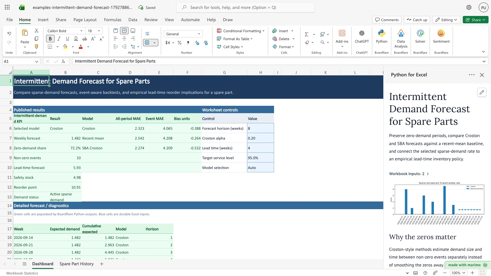
Dashboard: The primary planning workspace.Dashboard!G5:H10: Worksheet controls table for setting forecast horizon, Croston alpha, lead time, target service level, and model selection.Dashboard!A5:B13: Key performance indicator summary (summaryoutput), showing the selected model, weekly demand rate, zero-demand share, non-zero events, lead-time forecast, safety stock, reorder point, and demand status.Dashboard!C5:F10: Model evaluation & backtest comparison table (comparisonoutput), comparing All-period MAE, Event MAE, and Bias units across Croston, SBA Croston, and Recent mean.Dashboard!A17:E33: Forward forecast table (forecastoutput), providing multi-week expected demand and cumulative projections up to 16 weeks ahead.
Spare Part History: The raw demand history sheet.Spare Part History!A5:B1000: Historical weekly table withWeekandDemand units. The first 36 rows contain baseline sample data, followed by preformatted input rows through row 108. The notebook reads up to row 1000 and automatically ignores trailing empty rows.
| Worksheet | Range | Description | Type |
|---|---|---|---|
Dashboard |
G5:H10 |
Planning controls (horizon, alpha, lead time, service level, model override) | Editable inputs |
Dashboard |
A5:B13 |
Key inventory KPIs, replenishment thresholds, and demand status | Published output |
Dashboard |
C5:F10 |
One-step-ahead backtest error metrics by candidate model | Published output |
Dashboard |
A17:E33 |
Forward weekly forecast and cumulative expected demand | Published output |
Spare Part History |
A5:B1000 |
Weekly demand history (dates and unit counts) | Editable inputs |
Using the template
1. Update demand history
Paste or enter consecutive weekly demand observations into Spare Part History!A5:B1000. Enter dates at 7-day intervals and keep zero-demand weeks explicit as 0. The notebook dynamically ignores blank rows below the populated history.
2. Configure planning assumptions
On the Dashboard worksheet under Worksheet controls: - Adjust Forecast horizon (weeks) (from 1 to 16 weeks). - Adjust Croston alpha (typically 0.10 to 0.30; default 0.20). - Enter supplier Lead time (weeks) (e.g., 4 weeks). - Specify the Target service level (e.g., 95.0%). - Keep Model selection on Auto to let the backtest choose the most accurate method, or pick an explicit model from the dropdown.
3. Review model selection and backtest accuracy
Review the Published results comparison table (Dashboard!C5:F10). Auto selection prioritizes Event MAE first, absolute signed bias second, and all-period MAE third, ensuring that zero-heavy periods do not distort method selection.
4. Review inventory recommendations and demand status
Examine the KPI summary table (Dashboard!A5:B13): - Check the Weekly forecast and total Lead-time forecast. - Review Safety stock and the resulting Reorder point. - Monitor the Demand status indicator. If the trailing run of zero-demand periods exceeds twice Croston’s smoothed inter-demand interval, the status changes from Active sparse demand to Review obsolescence.
Inputs and settings
| Input / Column | Range | Allowed values | Default | Description |
|---|---|---|---|---|
Forecast horizon (weeks) |
Dashboard!H6 |
Integer 1 to 16 | 8 | Number of forward weekly periods projected in the forecast table. |
Croston alpha |
Dashboard!H7 |
Number in (0, 1] | 0.20 | Exponential smoothing parameter balancing responsiveness against noise. |
Lead time (weeks) |
Dashboard!H8 |
Positive integer (\(\ge 1\)) | 4 | Supplier replenishment lead time in weeks. |
Target service level |
Dashboard!H9 |
Percentage in [50%, 100%) | 95.0% | Desired non-stockout probability during replenishment lead time. |
Model selection |
Dashboard!H10 |
Auto, Croston, SBA Croston, Recent mean |
Auto |
Selects the forecasting method used for forward projections and safety stock. |
Week |
Spare Part History!A5:A1000 |
Date (7-day spacing) | Sample dates | Week start date. Must be unique and consecutive. |
Demand units |
Spare Part History!B5:B1000 |
Non-negative integer (\(\ge 0\)) | Sample counts | Units demanded during that week. Zeros must be explicit. |
How results are calculated
- Data cleaning and validation: Populated rows from
Spare Part History!A5:B1000are stripped of blank entries, sorted, and checked for unique consecutive 7-day dates. The series must have at least 20 periods and three non-zero demand events. - Croston’s method:
- Decomposes intermittent demand into two separate series: demand size when demand occurs (\(z\)) and inter-arrival interval between demand events (\(p\)).
- When demand \(y_t > 0\), with elapsed intervals \(q_t = t - t_{\text{last}}\): \[z_t = \alpha y_t + (1 - \alpha) z_{t-1}\] \[p_t = \alpha q_t + (1 - \alpha) p_{t-1}\]
- When \(y_t = 0\), both smoothed levels remain unchanged.
- The weekly demand rate forecast is \(\hat{y} = z_t / p_t\).
- Syntetos-Boylan Approximation (SBA):
- Classic Croston has an inherent positive bias because the ratio of expected values does not equal the expected value of ratios (\(E[z/p] > E[z]/E[p]\)).
- SBA applies a multiplicative deflator: \(\hat{y}_{\text{SBA}} = (1 - \alpha / 2) \cdot (z_t / p_t)\).
- Recent-mean baseline:
- Computes the unweighted arithmetic mean of the trailing 12 historical periods: \(\hat{y}_{\text{mean}} = \frac{1}{12} \sum_{i=0}^{11} y_{T-i}\).
- Event-aware rolling backtest:
- Evaluates one-step-ahead forecasts over the trailing 12 historical periods (periods 24 to 35).
- Computes All-period MAE, Event MAE (MAE on periods where actual demand \(y > 0\)), and signed Bias units (\(\text{forecast} - \text{actual}\)).
- Auto selection ranks candidate models by lowest Event MAE first, lowest absolute bias second, and lowest all-period MAE third.
- Empirical lead-time error calibration:
- Rather than relying on standard Gaussian safety stock formulas that assume normality and fail on zero-inflated demand, the model calculates rolling lead-time errors over all historical origins with at least 3 prior demand events.
- For each historical origin \(t\), forecast lead-time demand is \(\hat{Y}_{t, L} = \hat{y}_t \times L\), and actual lead-time demand is \(Y_{t, L} = \sum_{k=1}^L y_{t+k}\).
- Forecast error is \(e_t = Y_{t, L} - \hat{Y}_{t, L}\).
- Safety stock is calculated as the empirical quantile: \(\text{SS} = \max(0, \text{Quantile}(e, \text{service\_level}))\).
- Reorder point: \(\text{ROP} = (\hat{y} \times L) + \text{SS}\).
- Obsolescence monitoring:
- Tracks the trailing run of zero-demand periods: \(r = T - 1 - t_{\text{last}}\).
- If \(r > 2 \times p_T\) (the trailing zero run exceeds twice Croston’s smoothed inter-demand interval), demand status is flagged as
Review obsolescence; otherwise,Active sparse demand.
Worked example with sample data
- History profile: 36 weeks of history, 10 non-zero demand events, 26 zero-demand weeks (72.22% zero share).
- Croston levels: Trailing smoothed demand size \(z = 5.412\) units; smoothed interval \(p = 3.652\) weeks.
- Weekly rate: \(5.412 / 3.652 = 1.482\) units/week.
- SBA rate: \(1.482 \times (1 - 0.20 / 2) = 1.333\) units/week.
- 12-period backtest results:
- Croston: Event MAE = 4.065, All-period MAE = 2.323, Bias = -0.388 units.
- Recent mean: Event MAE = 4.208, All-period MAE = 2.542, Bias = -0.264 units.
- SBA Croston: Event MAE = 4.209, All-period MAE = 2.274, Bias = -0.532 units.
- Croston achieves the lowest Event MAE (4.065) and is selected by Auto.
- Lead-time forecast: At a 4-week lead time, \(1.482 \times 4 = 5.93\) units.
- Safety stock & reorder point: Applying the 95.0% quantile to rolling 4-week errors yields 4.98 units of safety stock and a reorder point of \(5.93 + 4.98 = 10.91\) units.
- Obsolescence check: The last demand event occurred at week 34 (0-indexed); trailing zero run is 1 week. The threshold is \(2 \times 3.652 = 7.30\) weeks. Since \(1 \le 7.30\), status is
Active sparse demand.
Reading the results
- Summary KPI table (
Dashboard!A5:B13):Selected model: Active forecasting method (Croston).Weekly forecast: Expected demand rate per week (1.482 units).Zero-demand share: Proportion of zero-demand periods in history (72.2%).Non-zero events: Total demand occurrences in history (10).Lead-time forecast: Expected demand during supplier lead time (5.93 units).Safety stock: Buffer units required to meet target service level (4.98 units).Reorder point: Inventory replenishment trigger level (10.91 units).Demand status: Operational diagnostic (Active sparse demandorReview obsolescence).
- Model comparison table (
Dashboard!C5:F10):- Compares candidate models across All-period MAE, Event MAE, and Bias units.
- Forward forecast table (
Dashboard!A17:E33):- Detailed weekly projections:
Week,Expected demand,Cumulative expected,Model,Horizon.
- Detailed weekly projections:
- Task pane chart:
- Visualizes observed weekly demand bars over the trailing 20 weeks alongside the forward weekly rate line.
- Diagnostic guidance:
- If safety stock is 0.00, historical lead-time demand never exceeded forecasts at the target service level.
- If demand status flags
Review obsolescence, investigate whether the part is nearing end-of-life, being superseded by an engineering change, or experiencing extended stockout downstream.
Saving, sharing and App mode
- Workbook persistence: Saving the
.xlsxfile stores all input history, controls, and generated output cells. Reopening the workbook retains all values. - Multi-user collaboration: Other users can view and edit the workbook in Excel. The Python backend evaluates deterministically whenever inputs change.
- App mode: When opened in Boardflare App mode, the task pane focuses on the interactive chart, model selection summary, and operational diagnostics, hiding authoring controls. App mode is a presentation layer designed for planner usability, not a security boundary or permissions control.
Errors, empty states and limits
- Error conditions and remedies:
- “Each populated history row must contain both a week and demand units; blank rows are ignored.”: Ensure every populated row has both a valid date and a numeric unit count.
- “Demand history must contain unique weekly dates.”: Eliminate duplicate weeks in
Spare Part History!A5:A1000. - “Demand history must use consecutive weekly dates with seven-day spacing.”: Verify calendar weeks have no gaps or irregular intervals.
- “Intermittent-demand history requires at least 20 non-negative periods and three non-zero events.”: Ensure at least 20 weeks of data are provided with at least 3 non-zero demand events.
- “Forecast horizon must be an integer from 1 to 16 weeks.”: Adjust horizon between 1 and 16.
- “Lead time must be a positive whole number of weeks.”: Set lead time to an integer \(\ge 1\).
- “Croston alpha must be in (0, 1].”: Enter a smoothing factor greater than 0 and less than or equal to 1.
- “Target service level must be at least 50% and below 100%.”: Specify service level as a decimal between 0.50 and 0.999.
- “Model selection must be Auto, Croston, SBA Croston, or Recent mean.”: Select a supported method name.
- “History does not provide at least five lead-time forecast-error samples after the third demand event.”: Provide additional historical weeks to accumulate at least 5 rolling lead-time evaluation windows.
- Empty state: The workbook includes 36 weeks of valid sample history. Clearing all data below the minimum threshold displays a descriptive error in the task pane.
- Hard limits: The history range reads up to row 1000 (
A5:B1000). The forecast spill table accommodates up to 16 weeks (A17:E33).
Limitations and when to use this
- Scope: Designed specifically for slow-moving, intermittent, and lumpy spare parts inventory where demand is zero in many periods.
- Limitations:
- Single-item model: Evaluates one SKU at a time; does not aggregate across multi-item hierarchies or item classes.
- Empirical error estimation requires sufficient history; short histories with few events can produce noisy safety stock estimates.
- Obsolescence alert is a diagnostic threshold flag (\(2 \times \hat{p}\)), not an automated Bayesian decay model.
- Assumes deterministic replenishment lead time; does not account for supplier lead-time variability, batch order quantities (MOQ / EOQ), or capacity constraints.
- When to use: Use when standard moving averages or exponential smoothing severely underestimate variability due to zero inflation, and when stockout costs warrant empirical safety stock protection.
Developer reference
Notebook implementation
The notebook reads demand history and worksheet controls from the workbook, cleans and validates inputs, defines forecasting methods in a modular reactive cell, performs an expanding-window backtest, evaluates empirical lead-time quantile errors, and publishes results via bf.publish.
Inputs are bound using bf.inputs:
inputs = bf.inputs(
    history=bf.ref("Spare Part History!A5:B1000", headers=True),
    controls=bf.ref("Dashboard!G5:H10", headers=True),
)
Core forecasting algorithms are implemented as pure functions: - croston_state(values, alpha) tracks the exponentially smoothed demand level \(z\) and inter-demand interval \(p\). - croston_rate(values, alpha, corrected=False) returns \(z / p\) (or \((1 - \alpha/2) \cdot z / p\) for SBA). - recent_mean(values) calculates the simple mean of the trailing 12 periods.
Outputs are published to designated workbook ranges:
publication = bf.publish(outputs={
    "summary": summary,
    "comparison": comparison,
    "forecast": forecast,
})
How the calculation/model works
Croston exponentially smooths non-zero demand size and inter-demand interval separately, then divides the two estimates to obtain a weekly demand rate. SBA applies the common (1 − α/2) correction to reduce Croston’s positive bias. A recent 12-period rolling one-step backtest reports all-period MAE, non-zero-event MAE, and signed unit bias. Auto selection ranks event MAE first, absolute bias second, and all-period MAE third, preventing zero-heavy all-period error from being the primary decision rule. The worksheet model selection can override Auto.
For the selected method, each eligible historical origin produces a lead-time forecast and an observed lead-time demand total. Forecast error is \(\text{actual lead-time demand} - \text{forecast lead-time demand}\). Safety stock is the chosen empirical service percentile of those rolling lead-time errors, floored at zero; reorder point is selected weekly demand \(\times\) lead time plus that safety stock. This avoids applying a Gaussian formula to raw zero-inflated weekly demand, although the empirical policy still depends on the amount and representativeness of available history.
Croston itself does not decay during a long run of zeros. The template therefore compares the trailing zero run with twice Croston’s smoothed inter-demand interval and surfaces Review obsolescence when that threshold is exceeded.
Validation / expected results
| Metric / Check | Expected outcome |
|---|---|
Selected model (Dashboard!B6) |
Croston |
Weekly forecast (Dashboard!B7) |
1.482 units |
Zero-demand share (Dashboard!B8) |
72.22% |
Non-zero events (Dashboard!B9) |
10 |
Lead-time forecast (Dashboard!B10) |
5.93 units |
Safety stock (Dashboard!B11) |
4.98 units |
Reorder point (Dashboard!B12) |
10.91 units |
Demand status (Dashboard!B13) |
Active sparse demand |
Croston All-period MAE (Dashboard!D6) |
2.323 units |
Croston Event MAE (Dashboard!E6) |
4.065 units |
- Appending a new demand event (5 units on week 2026-09-21) increases weekly forecast to 1.613 units, non-zero events to 11, zero share to 70.27%, and reorder point to 11.43 units.
- Reducing forecast horizon to 1 week restricts the forecast table to 1 row; expanding to 16 weeks extends projections through week 16 with 23.705 cumulative expected units.
- Varying Croston alpha to 0.05 lowers weekly forecast to 1.392 units (reorder point 10.31 units); increasing alpha to 0.90 adjusts weekly forecast to 1.149 units and safety stock to 5.98 units. Testing the upper bound alpha = 1.0 yields a 1.000 weekly rate, 4.00 lead-time forecast, 6.00 safety stock, and 10.00 reorder point.
- Selecting SBA Croston on the worksheet overrides automatic selection, applying the bias correction factor to produce a 1.333 weekly forecast, 5.49 safety stock, and 10.82 reorder point.
- Simulating a prolonged zero-demand run triggers the obsolescence diagnostic, changing demand status to
Review obsolescence.
Architecture
- Preallocated history input window:
Spare Part History!A5:B1000provides an oversized input range where trailing empty rows are stripped dynamically, allowing planners to paste new weekly observations without adjusting cell coordinates or formula ranges. - Horizon and spill synchronization: The
forecastoutput spills intoDashboard!A17:E33, exactly accommodating the maximum allowed 16-week horizon without overlapping adjacent worksheet sections. - Empirical lead-time error distribution: Rather than relying on standard Gaussian safety-stock formulas that fail on zero-inflated demand, safety stock is calibrated directly against empirical quantiles of rolling lead-time forecast errors.
Changelog
2026-10-23
- Modernized documentation to full 15-section application standard.
- Removed obsolete “Why Python” heading and restructured developer documentation under
## Developer referenceH3 subsections. - Verified Markdown table formatting and LaTeX math delimiter escaping.
- Refreshed workbook release artifacts and thumbnail poster.
2026-09-18
- Initial release with Croston and SBA forecasting, event-aware backtesting, and empirical lead-time safety stock (Issues #12, #21).