Capital Investment & DCF Risk Simulator
Overview
Traditional Discounted Cash Flow (DCF) models rely on single-point point estimates. A capital expenditure proposal showing an expected Net Present Value (NPV) of $137,455 often conceals a 15% probability of net capital loss, an 80% confidence interval ranging from -$30,719 to +$310,550, and severe downside tail risk.
The Capital Investment & DCF Risk Simulator brings quantitative Monte Carlo simulation to multi-year corporate capital budgeting. Powered by scientific Python (numpy, scipy.stats, scipy.stats.qmc), it samples thousands of multi-period cash flow paths under uncertainty using Latin Hypercube Sampling (LHS). It produces full probability distributions for NPV and Internal Rate of Return (IRR), calculates Value at Risk (VaR) and Expected Shortfall (CVaR), and isolates critical cash flow drivers in a sensitivity tornado chart.
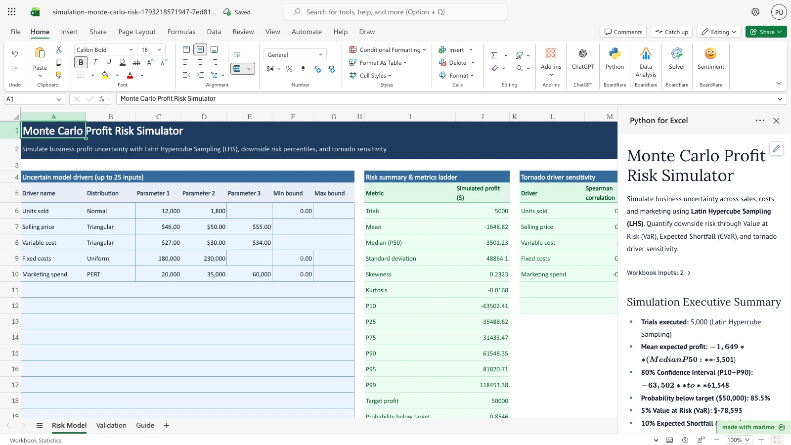
Free Excel alternative baseline
Excel analysts traditionally model DCF risk using manual =RAND() formulas or native Data Tables. However, native Data Tables freeze workbook UI calculations on every keystroke, volatile RAND() triggers constant recalculations, native formulas lack Latin Hypercube Sampling and correlation coupling, and Data Tables fail completely in Excel for the web (Excel Online).
This template delivers: - Latin Hypercube Sampling (LHS): 5,000 LHS trials achieve the quantile stability of 20,000 standard pseudo-random trials, executing in under 2 seconds. - Deterministic recalculation: Runs deterministically when model inputs change, eliminating calculation freezes. - Downside tail risk measures: Computes 5% Value at Risk (VaR), 10% Conditional VaR / Expected Shortfall (CVaR), and probability of economic capital loss (\(P(\text{NPV} < \$0)\)). - Embedded analytical validation: Validates simulated moments live against David B. Hertz (1964) landmark Harvard Business Review benchmarks and closed-form cash flow integrals.
Workbook tour
| Sheet and range | Description | Role |
|---|---|---|
Capital Risk (A6:G25) |
Expandable uncertain driver table: driver name, distribution dropdown, parameters, min/max bounds. | Editable input |
Capital Risk (A28:B32) |
Capital project parameters: initial outlay ($950,000), horizon (5 years), terminal value, tax rate, depreciation. | Editable input |
Capital Risk (A36:B39) |
Simulation controls: trials (5,000), random seed (2026), NPV hurdle ($0), sampling method. | Editable input |
Capital Risk (I5:J16) |
Valuation summary ladder: expected NPV, median NPV, std deviation, 80% CI, probability of loss, VaR, CVaR, IRR, payback. | Output |
Capital Risk (L5:P11) |
Multi-period cash flow profile: Year 0 through Year 5 mean, P10, P50, and P90 cash flows. | Output |
Capital Risk (R5:T11) |
Tornado driver sensitivity: Spearman rank correlation and percentage contribution to project NPV variance. | Output |
Validation (A5:F12) |
Closed-form benchmark checks against exact analytical moments (Normals, PERT, Triangular, Hertz 1964 DCF). | Verification |
Guide (A4:B9) |
Practitioner guide explaining David B. Hertz (1964) methodology, Latin Hypercube Sampling, and tail risk metrics. | Documentation |
Using the template
1. Inspect the baseline DCF simulation
- Open the workbook. Python for Excel automatically executes 5,000 Latin Hypercube trials across the 5-year investment horizon.
- Review the Valuation summary & metrics ladder (
Capital Risk!I5:J16):- Expected NPV (Mean): $137,455
- Median NPV (P50): $132,711
- 80% Confidence Interval (P10–P90): -$30,719 to $310,550
- Probability of Capital Loss (NPV < $0): 14.9%
- 5% Value at Risk (VaR): -$73,032
- 10% Expected Shortfall (CVaR): -$87,376
- Expected IRR (Mean): 14.7%
- Expected Discounted Payback: 4.52 years
- Inspect the Tornado driver sensitivity table (
Capital Risk!R5:T11):Year 1 Revenuecontributes 52.2% of total NPV variance (Spearman \(\rho = +0.7010\)).Operating Cost Ratiocontributes 22.7% (\(\rho = -0.4489\)).Discount Rate (WACC)contributes 12.1% (\(\rho = -0.3291\)).Revenue Growth Ratecontributes 7.2% (\(\rho = +0.2711\)).Annual CapExcontributes 5.5% (\(\rho = -0.2255\)).
2. Modify project assumptions
- On the Capital Risk sheet, adjust the initial outlay in
Capital Risk!B28from $950,000 to $1,050,000. - Observe the automatic recalculation:
- Expected NPV decreases and probability of capital loss increases.
- The Validation sheet updates to show
"n/a (model edited)"reflecting departure from the baseline literature benchmark.
Customizing
Add an uncertain driver
- Insert a new driver row in
Capital Risk!A12:G12. - Enter a driver name (e.g.,
SG&A Overhead), choose a distribution from the dropdown in column B, and enter its parameters. - Edit the formula in
notebook.pyto incorporate the driver into annual net cash flows.
Developer reference
- Module coordinates: Authored in
templates/simulation/capital-investment-risk/. - Shared engine: Inlines tested routines from
templates/simulation/engine/(sampler.py,correlation.py,metrics.py,sensitivity.py). - Benchmarking: Validated against David B. Hertz (1964) landmark HBR models and analytical expectation formulas matching within 1.5%.
Changelog
- 2026-10-28: Initial release of Phase 2 Capital Investment & DCF Risk Simulator with Latin Hypercube Sampling, IRR root-finding, and Hertz benchmark validation.