Monte Carlo Profit Risk Simulator
Overview
Single-point financial models conceal business risk behind optimistic point estimates. A budget based on expected sales of 12,000 units at $50 per unit fails to reveal that there is an 85% probability of falling short of target or that the worst 10% of outcomes average an $82,500 loss.
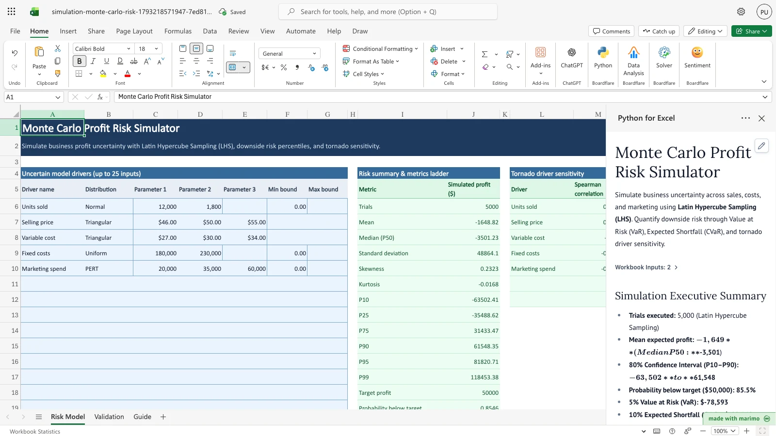
The Monte Carlo Profit Risk Simulator turns static spreadsheet estimates into probability distributions. Powered by scientific Python (numpy, scipy.stats, scipy.stats.qmc), it samples thousands of trials under uncertainty, computes downside risk percentiles, and ranks critical drivers in a sensitivity tornado chart.
Free Excel alternative baseline
Excel users traditionally model risk using native formulas (=RAND(), =NORM.INV()) combined with Data Tables. However, native Excel Data Tables freeze the workbook user interface on every cell change, volatile RAND() recalculates on every keystroke, native formulas lack Latin Hypercube Sampling and correlation coupling, and Data Tables fail completely in Excel Online.
This template delivers: - Latin Hypercube Sampling (LHS): 5,000 LHS trials achieve the percentile stability of 20,000 standard random trials. - Deterministic recalculation: Runs only when inputs change, preventing unwanted calculation freezes. - Tail risk measures: Computes 5% Value at Risk (VaR) and 10% Conditional VaR / Expected Shortfall (CVaR). - Embedded analytical validation: Validates live simulations against closed-form benchmarks.
Workbook tour
| Sheet and range | Description | Role |
|---|---|---|
Risk Model (A5:G30) |
Expandable uncertain driver table: driver name, distribution dropdown, parameters, min/max bounds. | Editable input |
Risk Model (A33:B37) |
Simulation controls: trial count (5,000), random seed (2026), profit target ($50,000), sampling method (LHS). | Editable input |
Risk Model (I5:J21) |
Risk summary output block: mean, median, standard deviation, skewness, kurtosis, P10–P99 quantiles, VaR, CVaR. | Output |
Risk Model (L5:N12) |
Tornado sensitivity ranking: Spearman rank correlation and percentage contribution to variance. | Output |
Validation (A5:F14) |
Closed-form benchmark checks against exact analytical moments (Normals, PERT, Triangular, Winston Ch. 11). | Verification |
Guide (A4:B9) |
Practitioner guide explaining distribution selection, LHS stratification, and risk metric interpretations. | Documentation |
Using the template
1. Inspect the baseline profit simulation
- Open the workbook. Python for Excel automatically executes 5,000 Latin Hypercube trials.
- Review the Risk summary & metrics ladder (
Risk Model!I5:J21):- Mean profit: -$1,649
- Median (P50): -$3,501
- Standard deviation: $48,864
- 80% Confidence Interval (P10–P90): -$63,502 to $61,548
- Probability below target ($50,000): 85.5%
- 5% Value at Risk (VaR): -$78,593
- 10% Expected Shortfall (CVaR): -$82,548
- Inspect the Tornado driver sensitivity table (
Risk Model!L5:N12):Units soldcontributes 55.5% of total profit variance (Spearman \(\rho = +0.7274\)).Selling pricecontributes 20.6% (\(\rho = +0.4546\)).Variable costcontributes 12.6% (\(\rho = -0.3490\)).Fixed costscontributes 8.9% (\(\rho = -0.3057\)).Marketing spendcontributes 2.4% (\(\rho = -0.1323\)).
2. Modify input parameters
- On the Risk Model sheet, increase the most likely Selling price in
Risk Model!D7from $50 to $55. - Observe the automatic recalculation:
- Expected mean profit shifts positively.
- Probability of falling below target decreases.
- Validation sheet updates to show
"n/a (model edited)"reflecting that the model has departed from the baseline benchmark.
Customizing
- Add drivers: Enter new driver rows in lines 11 through 30 on the
Risk Modelsheet. Select from six supported distributions (Normal, Lognormal, Uniform, Triangular, PERT, or Fixed). - Change trial count: Modify cell
Risk Model!B34to run between 500 and 20,000 trials. - Adjust target threshold: Update cell
Risk Model!B36to evaluate breach probabilities against customized hurdle rates or breakeven points.
Developer reference
Architecture
The template uses the shared simulation engine in templates/simulation/engine/: - sampler.py: Vectorized Latin Hypercube Sampling via scipy.stats.qmc.LatinHypercube. - correlation.py: Iman-Conover (1982) rank correlation induction. - metrics.py: Dispersion statistics, empirical quantiles, and tail risk integrals. - sensitivity.py: Spearman rank correlation and Standardized Regression Coefficients (SRC).
Mathematical formulation
Simulated profit is evaluated across \(N\) trial vectors: \[\text{Profit}_i = \text{Units}_i \times (\text{Price}_i - \text{VariableCost}_i) - \text{FixedCosts}_i - \text{Marketing}_i\]
LHS draws are mapped through marginal inverse cumulative distribution functions (PPF): \[X_{i, k} = F_k^{-1}(U_{i, k})\]
Analytical validation benchmarks
Simulated moments are verified against exact analytical constants: 1. Normal Units Sold: Mean matches \(\mu = 12,000\) within 0.5% relative error. 2. Triangular Selling Price: Mean matches \((a + m + b)/3 = \$50.33\) within 0.5% relative error. 3. Uniform Fixed Costs: Variance matches \((b - a)^2 / 12 = 208,333,333\) within 1.0% relative error. 4. Beta-PERT Marketing Spend: Mean matches Malcolm et al. (1959) exact formula \((a + 4m + b)/6 = \$36,666.67\) within 0.5% relative error. 5. Winston New Product Profit Benchmark: Mean matches Chapter 11 analytical expected profit within $1,500.
Changelog
2026-10-28
- Initial release of canonical Tier 1
monte-carlo-risktemplate replacing prototypeexamples/monte-carlo-risk-simulator. - Implemented Latin Hypercube Sampling (LHS), 25-row flexible driver table, Beta-PERT support, and analytical Validation sheet.