Project Cost & Contingency Risk Simulator
Overview
Traditional capital project budgets add an arbitrary flat contingency markup—typically 10% or 15%—across all cost line items. This practice underprotects high-uncertainty civil and structural work packages while locking up excess capital in fixed-fee scopes.
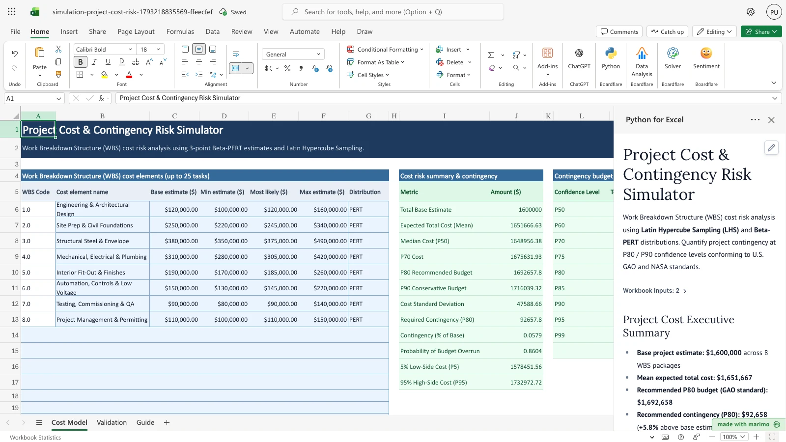
The Project Cost & Contingency Risk Simulator applies quantitative Monte Carlo risk analysis to an expandable Work Breakdown Structure (WBS). Using 3-point Beta-PERT estimates and Latin Hypercube Sampling (LHS), it generates the full project cost S-curve (cumulative distribution function), establishes defensible budget contingency at the 80th percentile (P80) per U.S. GAO and NASA standards, and isolates critical cost drivers in a sensitivity tornado chart.
Free Excel alternative baseline
Traditional Excel project cost contingency relies on manual =RAND() formulas or flat percentage markups. Flat markups ignore line-item variance differences, while volatile =RAND() recalculates on every cell edit. Native Excel Data Tables freeze recalculations, lack Latin Hypercube Sampling, and fail in Excel Online.
This template delivers: - Latin Hypercube Sampling (LHS): Efficient variance reduction ensuring accurate P80/P90 tail estimates with 5,000 trials. - Beta-PERT distributions: Avoids the excessive weight Triangular distributions place on corner estimates (Malcolm et al. 1959). - GAO-aligned contingency ladder: Explicit budget tiers from P50 median to P99 conservative cap. - Analytical validation: Dedicated validation sheet benchmarking simulated moments against exact Polaris PERT closed-form formulas.
Workbook tour
| Sheet and range | Description | Role |
|---|---|---|
Cost Model (A5:G30) |
Work Breakdown Structure (WBS) table: WBS code, task name, base estimate, 3-point min/mode/max estimates, distribution. | Editable input |
Cost Model (A33:B37) |
Simulation controls: trial count (5,000), random seed (2026), contingency confidence target (80% / P80), sampling method (LHS). | Editable input |
Cost Model (I5:J17) |
Cost risk summary: total base estimate, expected cost, P80 recommended budget, required contingency dollar amount, and overrun probability. | Output |
Cost Model (L5:O15) |
Contingency confidence ladder: P50 to P99 budget tiers, contingency dollars, and contingency percentage of base estimate. | Output |
Cost Model (Q5:S14) |
Critical cost driver sensitivity: Spearman correlation and percentage contribution to project cost variance. | Output |
Validation (A5:F13) |
Closed-form benchmark checks against exact Malcolm et al. (1959) and NASA CEH Appendix G analytical formulas. | Verification |
Guide (A4:B9) |
Practitioner guide explaining GAO Cost Estimating Guide standards, PERT mathematics, and contingency policies. | Documentation |
Using the template
1. Inspect the baseline WBS cost simulation
- Open the workbook. Python for Excel executes 5,000 Latin Hypercube trials across the 8 WBS packages.
- Review the Cost risk summary & contingency block (
Cost Model!I5:J17):- Total Base Estimate: $1,600,000
- Expected Total Cost (Mean): $1,651,667
- Median Cost (P50): $1,648,956
- P80 Recommended Budget (GAO Standard): $1,692,658
- Required Contingency (P80): $92,658 (+5.8% above base estimate)
- Probability of Budget Overrun: 86.0%
- Inspect the Critical cost driver sensitivity table (
Cost Model!Q5:S14):3.0 Structural Steel & Envelopecontributes 24.4% of total project cost variance.4.0 Mechanical, Electrical & Plumbingcontributes 24.4%.2.0 Site Prep & Civil Foundationscontributes 18.6%.- Together, the top three work packages drive 67.4% of total budget uncertainty.
2. Adjust contingency confidence target
- On the Cost Model sheet, locate cell
Cost Model!B36(Contingency target). - Increase the target from 80% (
0.80) to 90% (0.90). - Observe the immediate recalculation:
- Summary metric shifts to
Required Contingency (P90). - Recommended contingency amount increases to $116,039 (+7.3% above base).
- Summary metric shifts to
Customizing
- Add WBS work packages: Enter up to 25 tasks in rows 13 through 30 on the
Cost Modelsheet. - Select distributions: Use the in-cell dropdown in column G to switch individual work packages between PERT, Triangular, or Fixed cost.
- Change trial count: Modify cell
Cost Model!B34to evaluate larger trial samples (up to 20,000 trials).
Developer reference
Architecture
The template uses the shared simulation engine in templates/simulation/engine/: - sampler.py: Vectorized Beta-PERT and Triangular sampling via scipy.stats.beta and scipy.stats.qmc. - metrics.py: Percentile ladders, overrun probabilities, and dispersion statistics. - sensitivity.py: Spearman rank correlation and variance contribution share for WBS elements.
Mathematical formulation
Total project cost is the sum of stochastic WBS components: \[\text{Cost}_i = \sum_{j=1}^{K} X_{i, j}\]
Each work package follows a 4-parameter Beta-PERT distribution over \([a_j, b_j]\) with mode \(m_j\): \[\mu_j = \frac{a_j + 4m_j + b_j}{6}, \quad \sigma_j^2 = \frac{\alpha_j \beta_j (b_j - a_j)^2}{252}\]
Analytical validation benchmarks
Simulated moments are verified against exact analytical constants: 1. Polaris PERT Sum (Mean): Expected total project cost matches \(\sum \mu_j = \$1,651,666.67\) within 0.5% relative error. 2. Polaris PERT Sum (Std Dev): Total project cost standard deviation matches exact \(\sqrt{\sum \sigma_j^2} = \$48,415.37\) within 2.0% relative error. 3. Task 3.0 Structural Steel Mean: Matches \(\$390,000.00\) within 0.5% relative error. 4. Task 2.0 Civil Foundations Variance: Matches exact Beta-PERT variance within 1.5% relative error.
Changelog
2026-10-28
- Initial release of canonical Tier 1
project-cost-risktemplate. - Implemented 3-point Beta-PERT WBS roll-up, GAO P80 contingency calculation, cost S-curve, and Malcolm (1959) analytical validation benchmarks.