Workforce Volume Forecast
Forecast daily workload and translate it into staffing requirements without hiding operational assumptions inside Python. Historical volume determines the demand outlook; productivity, shrinkage, service buffer, and horizon remain editable in the workbook.
Result preview
The supplied ten-week history produces a 14-day workload forecast with 620.8 average volume, 729.9 peak volume, 11.57 average staffed shifts, and 14 peak staffed shifts. Before forecasting forward, a 14-day expanding-origin backtest records 1.30% WAPE versus 2.31% for a same-weekday seasonal-naive baseline.
What this template does
- Estimates a recent daily trend from historical workload.
- Backtests the model in temporal order against a same-weekday seasonal-naive forecast.
- Measures weekday seasonality from trend-adjusted residuals.
- Forecasts the next one to four weeks at daily granularity.
- Converts demand into staffed shifts using productivity, shrinkage, and service buffer.
- Summarizes weekday history, forecast averages, peak volume, and peak staffing.
Why Python
Weekday effects and trend can be implemented with formulas, but Python makes the decomposition, horizon generation, and staffing translation easier to inspect and extend. It also keeps the forecasting method separate from workforce policy controls, which remain visible in Excel.
Try it live
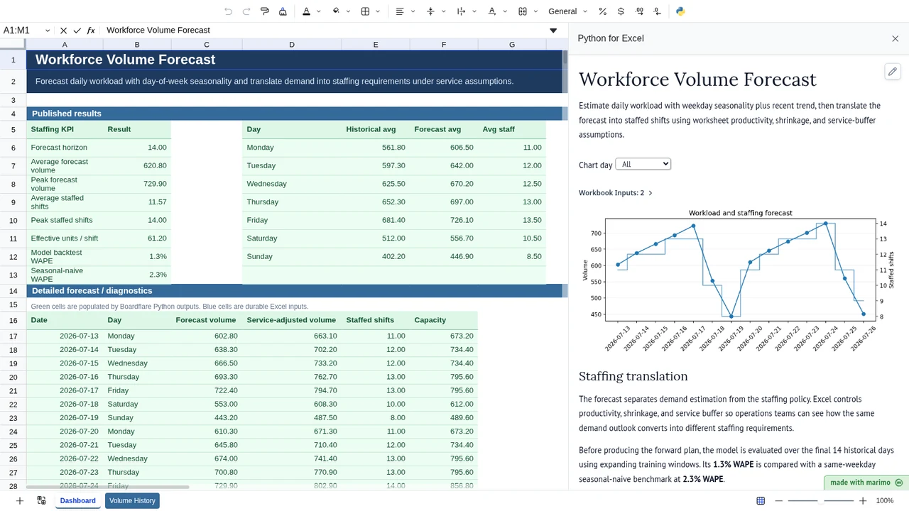
Change workload observations, shrinkage, productivity, service buffer, or forecast horizon and compare the resulting staffed-shift plan.
Operating workflow
Author: an operations analyst maintains the workload model, weekday/trend logic, staffing translation, validation, and published forecast outputs.
Workbook user: an operations manager updates recent volume and visible workforce assumptions such as productivity, shrinkage, service buffer, and horizon, then reviews the staffed-shift requirement.
For a recurring planning handoff, save the finished notebook to open in App mode and verify that a second user can complete the staffing review without author intervention. App mode simplifies presentation without hiding the saved source.
Download the Excel template
Inputs and assumptions
Volume History!A5:B75 contains 70 daily observations. Dashboard!J5:K9 contains a 14-day horizon, 72 units per staffed shift, 15% shrinkage, and a 10% service buffer. The model assumes each row represents one consecutive day and that the recent weekday pattern remains useful over the short forecast horizon.
Notebook implementation
bf.inputs(...) binds the daily history and staffing controls. The notebook publishes summary, weekday, and forecast tables while the notebook supplies a diagnostic weekday selector and workload/staffing visualization.
How the calculation/model works
A least-squares line estimates the overall daily trend. Residuals are averaged by weekday to estimate recurring day-of-week effects. Before fitting the final model, the last 14 historical days are evaluated one at a time with expanding training windows and compared with the observation from the same weekday one week earlier. Future workload then combines the full-history extrapolated trend with the appropriate weekday effect. Service-adjusted workload is forecast × (1 + service buffer). Effective staffed-shift capacity is units per shift × (1 − shrinkage), and required staffing is rounded up to the next whole staffed shift.
Validation / expected results
The baseline checks 620.8 average forecast volume, 729.9 peak forecast volume, 11.57 average staffed shifts, 14 peak staffed shifts, and 61.2 effective units per shift. It also verifies 1.30% model WAPE against 2.31% seasonal-naive WAPE over the final 14 historical days. A scenario increases shrinkage to 30% and verifies that forecast demand is unchanged while average staffing rises to 14.07, peak staffing to 16, and effective capacity falls to 50.4.
Limitations
The model does not account for intraday arrival curves, skill groups, shift lengths, queueing targets, holidays, promotions, weather, absenteeism, overtime rules, or integer scheduling constraints. Use it as a volume-to-staffing planning bridge rather than a finished shift scheduler.
When to use this approach
Use it when demand has a stable weekday pattern and operations needs a transparent short-horizon staffing estimate. If service levels depend on queues, handle times, or multi-skill routing, pair the volume forecast with a dedicated capacity or scheduling model.