Demand Forecast & Backtest Explorer
Use historical monthly demand to compare simple forecasting baselines before publishing a forward plan. The workbook keeps history, horizon, backtest depth, and interval width in Excel while Python for Excel handles rolling evaluation, model selection, and visualization.
Result preview
The supplied history is evaluated with seasonal-naive, three-month-average, and trend-plus-seasonality models. Trend + seasonality wins the baseline rolling-origin comparison with 9.25% WAPE and the first forward forecast is 1,406.90 units.
What this template does
- Preserves monthly demand history as editable worksheet inputs.
- Compares three understandable forecasting baselines rather than selecting a model by fit alone.
- Uses rolling-origin evaluation across multiple forecast steps.
- Reports WAPE, MAE, signed bias, and backtest point counts by model.
- Publishes the selected-model forecast and error-scaled lower/upper bands back to Excel.
Why Python
Forecast evaluation is naturally iterative: each backtest origin must recompute the model using only information that would have been available at that time. NumPy and pandas make that time-aware loop compact while keeping the workbook focused on durable data, assumptions, and decision outputs.
Try it live
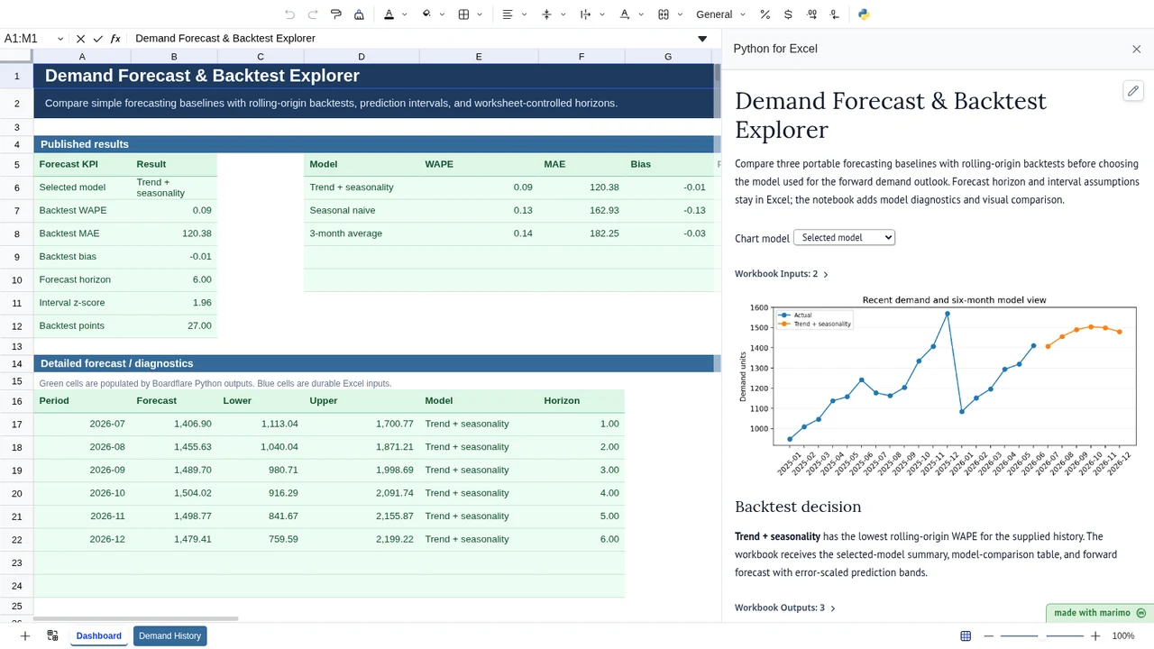
Change recent demand, forecast horizon, backtest origins, or interval z-score. The model comparison and forecast recalculate from the same worksheet state.
Operating workflow
Author: a demand-planning analyst maintains the history contract, candidate models, rolling-backtest logic, validation rules, and published forecast tables.
Workbook user: a planner updates demand history and durable forecast controls, then reviews the selected baseline, backtest metrics, and forward forecast without maintaining the Python implementation.
For repeated planning cycles, save the completed notebook to open in App mode and validate the same workbook with a second user. App mode simplifies the presentation but does not restrict access to the saved source.
Download the Excel template
Inputs and assumptions
Demand History!A5:B35 contains 30 monthly observations. Dashboard!J5:K8 contains the forecast horizon, number of rolling origins, and interval z-score. Demand must be non-negative and the history is assumed to be monthly and regularly spaced.
Notebook implementation
The notebook binds worksheet data and controls once, evaluates each candidate model over rolling origins, and publishes summary, comparison, and forecast worksheet tables with bf.publish(...). The notebook model selector changes only the diagnostic chart; durable forecast assumptions remain in Excel.
How the calculation/model works
Seasonal naive repeats the value from 12 months earlier. The three-month baseline carries the latest three-month mean forward. Trend + seasonality uses least squares on a time trend plus annual sine/cosine terms. Rolling origins score one- to three-step predictions where actuals are available. The selected model minimizes WAPE, with MAE as the tie-breaker. Prediction bands scale the selected model’s backtest residual standard deviation by z × √horizon.
Validation / expected results
The baseline asserts Trend + seasonality, 9.25% WAPE, 120.38 MAE, -0.75% bias, and a first forecast of 1,406.90. A worksheet-edit scenario changes the most recent demand to 1,800 and verifies 12.17% WAPE, 163.72 MAE, -3.95% bias, and a first forecast of 1,479.48 through the real Python for Excel runtime.
Limitations
These are intentionally transparent baselines, not a full automatic forecasting suite. The interval is an empirical residual band rather than a calibrated probabilistic forecast. Structural breaks, promotions, holidays, stockouts, missing periods, and explanatory variables are not modeled.
When to use this approach
Use it when a planning team needs a defensible baseline, wants to compare candidate forecasts with time-aware validation, or needs a benchmark before adopting a more complex forecasting method.