Intermittent Demand Forecast for Spare Parts
Model a spare part whose weekly history contains more zeros than demand events. The template keeps those zeros explicit, compares Croston-style forecasts with a recent-mean baseline, and turns the selected weekly rate into a lead-time forecast, safety stock, and reorder point.
Result preview
The supplied 36-week history is 72.22% zero-demand periods with 10 non-zero events. SBA Croston wins the holdout comparison, producing a 1.333-unit weekly forecast and a 13.92-unit reorder point.
What this template does
- Preserves sparse zero-demand periods instead of filtering them out.
- Implements classic Croston and SBA-corrected Croston forecasting.
- Compares sparse-demand methods with a recent-mean baseline.
- Reports both all-period and demand-event error metrics.
- Converts the selected weekly forecast into lead-time demand, safety stock, and reorder point.
Why Python
Croston methods maintain separate smoothed estimates for demand size and the interval between non-zero events. That stateful logic is cumbersome in ordinary spreadsheet formulas but concise in Python. Excel still owns the demand history and inventory-policy controls.
Try it live
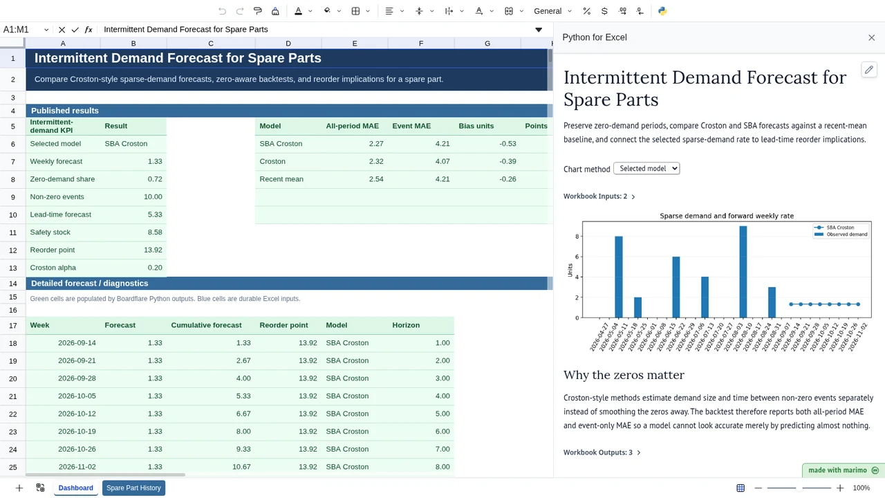
Edit zero/non-zero demand observations, smoothing alpha, lead time, service factor, or horizon to see the sparse-demand forecast and reorder point update.
Operating workflow
Author: an inventory analyst maintains the sparse-demand method, holdout evaluation, inventory-policy calculation, and validation rules.
Workbook user: a planner updates item history and visible policy assumptions such as smoothing, lead time, service factor, and horizon, then reviews the weekly forecast and reorder implication.
For a repeated spare-parts review cycle, the author can save the notebook to open in App mode and test the workbook with the planner who will operate it. App mode is a focused presentation, not a permissions boundary.
Download the Excel template
Inputs and assumptions
Spare Part History!A5:B41 contains 36 weekly observations including explicit zeros. Dashboard!J5:K9 contains an 8-week horizon, Croston alpha 0.20, 4-week lead time, and service z-score 1.65. The history must include at least three demand events.
Notebook implementation
The notebook reads history and controls through bf.inputs(...), computes candidate sparse-demand forecasts and holdout errors, and publishes summary, comparison, and forecast tables with bf.publish(...). The notebook method selector is diagnostic only.
How the calculation/model works
Croston exponentially smooths non-zero demand size and inter-demand interval separately, then divides the two estimates to obtain a weekly demand rate. SBA applies the common (1 − α/2) correction to reduce Croston’s positive bias. Rolling one-step forecasts over the latest 12 periods are scored with all-period MAE, non-zero-event MAE, and signed unit bias. Reorder point is modeled as selected weekly demand × lead time plus z × weekly demand standard deviation × √lead time.
Validation / expected results
The baseline checks SBA Croston, a 1.333 weekly forecast, 72.22% zero share, 10 demand events, 13.92 reorder point, and 2.274 selected all-period MAE. A scenario changes the latest zero week to 5 units and verifies a 1.551 weekly forecast, 69.44% zero share, 11 events, 14.97 reorder point, and 2.468 selected MAE.
Limitations
This is a single-item teaching model. The safety-stock formula uses raw weekly standard deviation and does not estimate service probability from an intermittent-demand distribution. It does not model obsolescence, repairables, censored stockout demand, multiple lead times, order quantities, or item pooling.
When to use this approach
Use Croston-style methods when demand events are sparse and a conventional moving average is dominated by zeros. For large spare-parts portfolios, evaluate methods by item class and connect the forecast to an inventory policy calibrated to service and holding-cost objectives.