Demand & Inventory Planner
Convert SKU demand, lead-time variability, cost, open orders, and durable worksheet planning controls into a budget-feasible replenishment plan. Unlike the earlier greedy allocation, this version solves an actual mixed-integer linear program so case-pack decisions are optimized together under one cash constraint.
Result preview
At the supplied 95%-style service factor (z = 1.65), 4-week horizon, 10-unit case pack, and $65,000 budget, the optimizer reaches Optimal status, confirms the plan is budget-feasible, funds $64,990 of purchases, and leaves $10 unallocated. Six SKUs begin below their reorder point and eight receive less than their full unconstrained replenishment requirement.
What this template does
- Calculates safety stock, reorder points, forecast demand, and unconstrained order requirements.
- Keeps budget, service z-score, horizon, and case pack as worksheet inputs in the workbook and live demo.
- Uses
scipy.optimize.milpfor integer case-pack purchase decisions under the cash budget. - Minimizes priority-weighted unfunded replenishment value rather than applying a row-by-row greedy rule.
- Publishes summary/detail outputs, solver status, a budget-feasibility check, and a reusable safety-stock function in Boardflare.
Why Python
The inventory math is vectorizable, but the shared budget plus integer case-pack decisions form a mixed-integer optimization problem. SciPy’s milp directly supports integral decision variables, bounds, and linear constraints, making the model easier to audit than a chain of spreadsheet allocation formulas. See the SciPy milp documentation.
Try it live
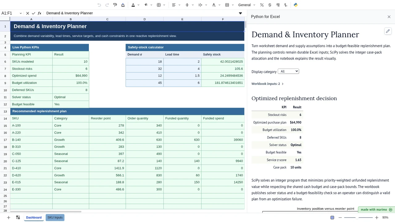
Edit SKU demand or any blue planning control on SKU Inputs. The optimized plan and notebook chart recompute from those same worksheet assumptions.
Operating workflow
Author: an inventory or supply-chain analyst maintains the optimization formulation, workbook input contract, validation scenarios, and published planning outputs.
Workbook user: a buyer or planner updates demand and visible planning controls such as budget, service factor, horizon, and case pack, then reviews the optimized order plan and deferred SKUs.
For a recurring purchasing workflow, save the completed notebook to open in App mode and have the intended operator run the same workbook independently. App mode focuses the presentation; it does not protect or remove the saved Python source.
Download the Excel template
Inputs and assumptions
The SKU table contains on-hand inventory, weekly demand, demand standard deviation, lead time, unit cost, and open purchase orders. J4:K8 contains the shared planning controls: cash budget, service z-score, planning horizon, and case pack.
Safety stock uses z × demand standard deviation × √lead time. This assumes the supplied weekly demand variability is appropriate for the modeled lead-time horizon and that a normal-approximation service factor is meaningful for the use case.
Notebook implementation
Boardflare uses the same worksheet inputs and the same SciPy formulation. The notebook adds a category display filter and visualization, while durable analytical controls remain in Excel.
inputs = bf.inputs(
    skus=bf.ref("SKU Inputs!A4:H14", headers=True),
    controls=bf.ref("SKU Inputs!J4:K8", headers=True),
)
solution = milp(...)
bf.publish(outputs={"summary": summary, "detail": detail})
How the calculation/model works
For each SKU, Python calculates forecast demand across the planning horizon, safety stock, reorder point, net available supply, and a case-pack-rounded unconstrained order. Priority is shortage requirement divided by reorder point. The MILP chooses an integer number of cases between zero and each SKU’s unconstrained maximum while total purchase cost stays within budget; the linear objective penalizes leaving higher-priority replenishment value unfunded.
SciPy represents the budget as a LinearConstraint; see the constraint documentation.
Validation / expected results
The baseline checks Optimal solver status, Yes budget feasibility, $64,990 optimized spend, 99.98% budget utilization, and 8 deferred SKUs. A lower-budget scenario sets the cash limit to $40,000 and verifies that the optimizer recomputes to $39,970 of spend with 10 deferred SKUs rather than returning cached output.
Limitations
This teaching model uses a common case pack and does not include supplier-specific MOQs, order timing, truck/container capacity, holding cost, shortage cost, quantity discounts, or correlated demand. The z-score is an input service factor, not a guaranteed fill rate. A production replenishment model should calibrate demand and service assumptions from historical data and add the constraints that actually govern purchasing.
When to use this approach
Use mixed-integer optimization when several replenishment decisions compete for one constrained budget and orders must respect discrete packs. If cash is not constraining or replenishment can be continuous, the optimization layer may be unnecessary.