Monte Carlo Profit Risk Simulator
Use reproducible Monte Carlo simulation to turn uncertain unit volume, selling price, variable cost, and fixed-cost assumptions into a profit distribution rather than a single-point plan.
Result preview
The canonical workbook runs 5,000 fixed-seed trials and reports mean profit, P10/P50/P90, probability of missing a worksheet profit target, average profit in the worst 10% of trials, and driver-to-profit sensitivity.
What this template does
- Reads uncertain driver distributions and simulation controls from Excel.
- Supports Normal, Triangular, Uniform, and Fixed inputs.
- Runs thousands of vectorized trials with a visible random seed.
- Publishes risk metrics, sensitivity ranking, and histogram bins into the workbook.
- Shows the full simulated profit distribution in the Python for Excel notebook.
Why Python
Monte Carlo simulation is compact in NumPy because one array represents thousands of trial values instead of thousands of worksheet rows. The template uses a seeded numpy.random.Generator for reproducibility, then derives normal and triangular samples from uniform draws with explicit transforms so the fixed fixture is less dependent on distribution implementation details across NumPy versions. NumPy documents default_rng as the recommended Generator constructor and also notes that the higher-level random stream is not guaranteed to remain bit-for-bit compatible across versions. See the NumPy random Generator documentation.
Try it live
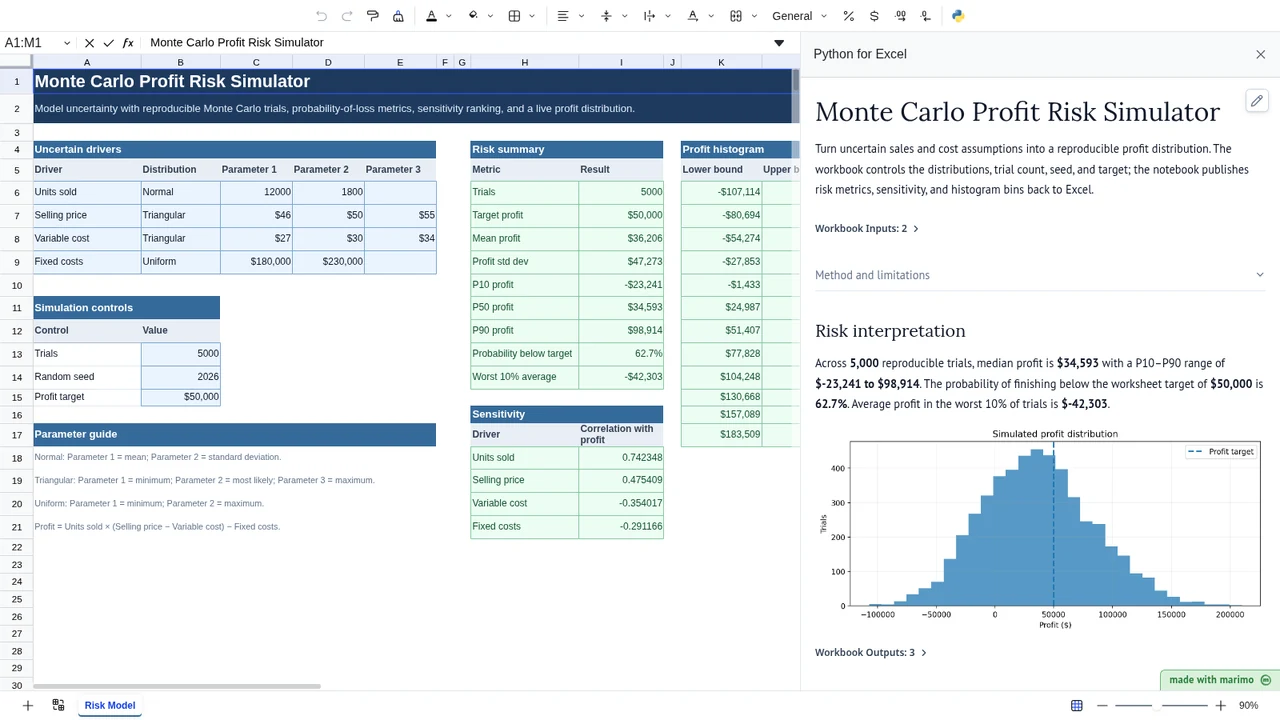
Change the variable-cost most-likely value, profit target, trial count, or seed. Published risk metrics and the notebook histogram recalculate from the worksheet state.
Operating workflow
Author: an FP&A or finance analyst maintains the uncertain-driver distributions, deterministic profit relationship, reproducibility controls, validation scenarios, and published risk diagnostics.
Workbook user: a finance manager updates visible assumptions such as ranges, most-likely values, trial count, profit target, or seed, then reviews downside probability, percentiles, and sensitivity before making a planning decision.
For a recurring planning handoff, save the finished notebook to open in App mode and verify that the intended operator can change assumptions and interpret the distribution without author intervention. App mode focuses presentation; it does not change workbook permissions, source access, or trust.
Download the Excel template
Inputs and assumptions
Risk Model!A5:E9 contains four uncertain drivers. Normal rows use mean and standard deviation, Triangular rows use minimum / most likely / maximum, and Uniform rows use minimum / maximum. Risk Model!A12:B15 contains trial count, seed, and target profit.
The deterministic profit relationship is:
Profit = Units sold × (Selling price − Variable cost) − Fixed costs
The first version assumes the four uncertain drivers are independent.
Notebook implementation
The notebook binds the input tables once, simulates the distributions, and publishes three worksheet-facing tables:
inputs = bf.inputs(
    drivers=bf.ref("Risk Model!A5:E9", headers=True),
    controls=bf.ref("Risk Model!A12:B15", headers=True),
)

bf.publish(outputs={
    "summary": summary,
    "sensitivity": sensitivity,
    "histogram": histogram,
})
How the calculation/model works
Each trial samples one value for each uncertain driver, then evaluates the same profit equation. P10, P50, and P90 are empirical quantiles of the resulting profit array. Probability below target is the share of trials below the workbook target. Worst-10% average is the mean of outcomes at or below P10. The histogram uses numpy.histogram, which returns trial counts for adjacent profit intervals. See the NumPy histogram documentation.
Sensitivity is the Pearson correlation between each sampled driver and profit. It is useful for screening which assumptions move with outcomes most strongly in this model, but it is not a causal effect estimate.
Validation / expected results
The offline release gate uses the fixed seed and checks selected baseline risk metrics directly in the real Boardflare/Univer runtime. It then raises the most-likely variable cost from $30 to $32 and verifies that the published profit distribution metrics recalculate to the scenario values in offline_test.py.
Limitations
Results are conditional on the selected distributions, parameters, deterministic profit equation, and independence assumption. A fixed seed makes the workbook reproducible; it does not make a probability estimate certain. Correlation sensitivity can also understate nonlinear or interaction effects. For consequential planning, calibrate assumptions from relevant historical or expert data and model material dependencies between drivers.
When to use this approach
Use Monte Carlo simulation when a decision depends on the range and probability of possible outcomes, not just a base-case value. It is particularly useful for budgets, projects, margins, capacity plans, and break-even analysis where several uncertain inputs compound.