Nonlinear Curve Fitting
Fit a realistic enzyme-kinetics dataset with SciPy rather than a nearly perfect synthetic curve. The default Michaelis-Menten model estimates a saturation rate and half-saturation constant, while worksheet controls select the model and prediction interval used by the Python for Excel notebook.
Result preview
For the supplied noisy observations, the default Michaelis-Menten fit produces approximately Vmax = 91.927 µmol/min, Km = 3.384 mM, RMSE = 0.844 µmol/min, R² = 0.99859, and a covariance condition number of about 363.
What this template does
- Reads measured substrate concentration and reaction-rate observations from Excel.
- Fits either Michaelis-Menten or power-law parameters with bounded
scipy.optimize.curve_fit. - Calculates RMSE, R², AIC, parameter standard errors, and covariance conditioning.
- Builds covariance-based prediction intervals and residual diagnostics.
- Publishes fit tables and a reusable prediction function back to Excel.
Why Python
Nonlinear parameter estimation, covariance diagnostics, interval calculations, and residual visualization are substantially easier to express and audit with SciPy and NumPy than with spreadsheet helper columns and Solver configuration. SciPy also documents important caveats around covariance reliability and conditioning that the template surfaces directly. See the scipy.optimize.curve_fit documentation.
Try it live
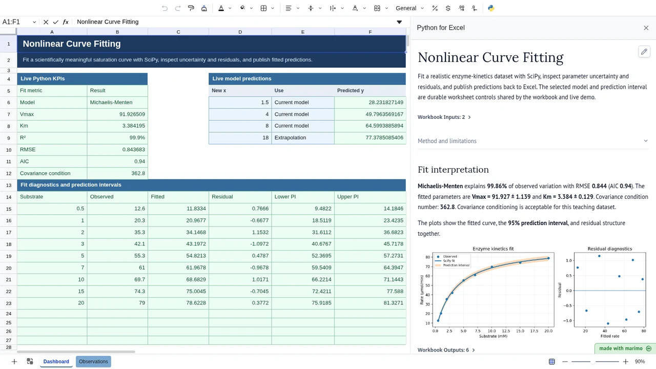
Edit a measured rate, change Model between Michaelis-Menten and Power law, or change the worksheet prediction interval. The fitted curve, diagnostics, and worksheet predictions all recompute from the same controls.
Operating workflow
Author: a technical analyst or engineer maintains the candidate equations, fitting/diagnostic logic, validation cases, and published prediction function.
Workbook user: a scientist or process engineer updates observations, selects the approved model and interval, then reviews fitted parameters, diagnostics, and worksheet predictions without editing the fitting code.
When this becomes a repeated review tool, the author can save the notebook to open in App mode and validate the workbook with its intended operator. App mode changes the visible authoring surface, not source availability.
Download the Excel template
Inputs and assumptions
Observations!A4:B13 contains substrate concentration in mM and observed rate in µmol/min. D4:E6 contains two durable fit controls: model choice and prediction interval. The default model is:
rate = Vmax × substrate / (Km + substrate)
The interval calculation treats residual errors as independent with roughly constant variance and uses a local-linearization approximation based on the fitted parameter covariance.
Notebook implementation
The Python for Excel notebook binds the same observations and worksheet controls, computes the same fit, then adds a two-panel visual diagnosis and publishes a live predict function:
inputs = bf.inputs(
    observations=bf.ref("Observations!A4:B13", headers=True),
    controls=bf.ref("Observations!D4:E6", headers=True),
)
parameters, covariance = curve_fit(...)
bf.publish(
    outputs={"summary": summary, "detail": detail},
    functions={"predict": predict},
)
How the calculation/model works
Nonlinear curve fitting estimates parameters for a chosen function so its predictions are close to observed data. For observations y and model predictions f(x, parameters), nonlinear least squares minimizes the sum of squared residuals. The canonical workbook fits the Michaelis-Menten saturation model, y = Vmax × x / (Km + x). Vmax is the asymptotic response and Km is the x-value at half that response.
curve_fit minimizes squared residuals to estimate the selected nonlinear parameters. The template then calculates residual variance, RMSE, R², AIC, standard errors from the returned covariance matrix, and numpy.linalg.cond(covariance) as a quick identifiability diagnostic. Prediction intervals combine local mean-response variance with residual variance.
Validation / expected results
For the canonical Michaelis-Menten model:
| Check | Expected value |
|---|---|
| Vmax | 91.926508 |
| Km | 3.384195 |
| RMSE | 0.843683 |
| R² | 0.998585 |
| AIC | 0.940386 |
| Covariance condition | 362.800 |
| Prediction at 8 mM | 64.599389 |
The offline pytest/Univer gate executes the canonical notebook.py in the real Boardflare browser runtime. It also changes the worksheet model to Power law and verifies the published fit metrics recalculate to the scenario values declared in offline_test.py.
Limitations
A high R² does not prove that Michaelis-Menten or any other candidate model is scientifically correct. The covariance and derived intervals are local approximations and can become unreliable when parameters are weakly identified or the covariance matrix is poorly conditioned. Predictions outside the measured concentration range are extrapolations. For formal inference, validate residual assumptions and use uncertainty methods appropriate to the experiment.
When to use this approach
Use nonlinear curve fitting when the functional form has scientific or operational meaning and the parameters themselves matter. If the primary goal is flexible prediction without a defensible functional form, consider a broader regression or machine-learning approach instead.