Optimization Toolbox
Beta · Optimization and global-search workbench for Python for Excel
Result preview
The Optimization Toolbox is a reusable optimization workbench, not a single-purpose Solver example. The workbook separates model definition, solver execution, solution review, and diagnostics so the same Excel structure can represent several classes of mathematical problems.
The Start sheet selects one of nine included models. The Variables, Linear Model, Quadratic & Conic, Expressions, and Scenarios sheets define the active mathematical model. The notebook then validates the model, classifies its structure, dispatches it to an appropriate Python solver, independently checks the returned decision vector, and publishes standardized results to Results, Analysis, and Diagnostics.
The default Product Mix — LP model maximizes contribution margin under labor, material, and demand limits. Its expected objective is 4,750, with 16.6667 chairs and 50 desks. The same workbook can then be switched to integer workforce scheduling, portfolio quadratic optimization, constrained nonlinear marketing allocation, nonlinear parameter estimation, nonlinear equations, a two-objective Pareto model, bounded multimodal global search, or a deliberately infeasible capacity model.
This beta is deliberately broader than the Examples elsewhere in the template library. Its purpose is to provide a durable modeling surface that can be deepened over time as additional solver families and diagnostics are validated in the browser runtime.
What this template does
Capability map
| Capability | Status | Current implementation |
|---|---|---|
| Linear programming | Available | SciPy HiGHS linprog with bounds, equalities, inequalities, ranged constraints, solver status, and constraint marginals |
| Mixed-integer linear programming | Available | SciPy HiGHS milp with continuous, integer, and binary variables |
| Quadratic objectives | Available | Shared quadratic model representation solved with constrained SLSQP; the included portfolio fixture is convex |
| Smooth constrained nonlinear optimization | Available | SLSQP with variable bounds, linear constraints, and safe worksheet-defined nonlinear constraints |
| Nonlinear least squares | Available | Weighted worksheet residuals solved with SciPy least_squares |
| Nonlinear equation systems | Available | Bounded equation residuals solved with least_squares and an explicit residual tolerance |
| LP marginal analysis | Available | HiGHS constraint marginals normalized to the workbook’s natural objective direction |
| Named scenarios | Available | Reusable overrides for parameters, variable bounds, linear-objective coefficients, and linear-constraint bounds |
| MultiStart | Available | Seeded repeated local solves with normalized comparison output |
| Differential Evolution | Available | Bounded stochastic global search with explicit seed and browser-scale evaluation budget |
| SHGO | Available | Deterministic bounded global search for the included unconstrained multimodal workflow |
| Local/global comparison | Available | Local SLSQP, MultiStart, Differential Evolution, and SHGO compared under one result contract |
| Two-objective Pareto analysis | Available | Epsilon-constraint frontier for two named linear objectives |
| Independent feasibility checking | Available | Returned decisions checked against bounds, integrality, linear constraints, and safe nonlinear constraints |
| Second-order cone programming | Planned | Requires a dedicated browser-runtime conic backend and validation gate |
| Dedicated QP solver and QP dual diagnostics | Planned | Current QP path uses the general smooth constrained optimizer |
| Classical LP allowable-range sensitivity | Planned | Current beta exposes local constraint marginals, not full RHS/objective ranging |
| Goal attainment / minimax | Planned | Current multiobjective implementation is epsilon-constraint rather than fgoalattain/fminimax parity |
| Surrogate optimization | Planned | Candidate for expensive black-box objectives after browser profiling |
| Pattern search | Exploring | Add when a derivative-free constrained local/direct-search workflow warrants it |
| Genetic algorithm / particle swarm / simulated annealing | Exploring | Not included merely to mirror MATLAB solver names; each needs a strong Excel use case and runtime gate |
| Automatic differentiation | Not available | The beta uses numerical derivatives provided by SciPy solvers |
| Parallel global optimization | Not available | Browser execution is intentionally single-worker |
Modules
The workbench is organized around six modules rather than around individual Python functions:
- Modeling — shared worksheet schemas for variables, parameters, objectives, constraints, quadratic terms, nonlinear expressions, and scenarios.
- Local and discrete optimization — LP, MILP, QP-style quadratic objectives, and smooth constrained NLP.
- Estimation and equations — nonlinear residual fitting and bounded nonlinear equation systems.
- Global search — bounded local/global comparison with deterministic and seeded stochastic methods.
- Tradeoff and scenario analysis — two-objective Pareto frontiers plus named what-if overrides.
- Diagnostics — structural validation, parser safety, feasibility checks, status normalization, scaling warnings, and solver evidence.
Documentation
The Toolbox has a fuller guide set than an ordinary Example:
- Getting started — first solve, changing models, running a scenario, and reading outputs.
- Modeling guide — complete worksheet schema, expression language, classification rules, and how to create a model.
- Solver guide — problem classes, solver selection, statuses, diagnostics, sensitivity, and MATLAB capability mapping.
- Global optimization guide — MultiStart, Differential Evolution, SHGO, reproducibility, and global-solution semantics.
- Worked examples — all nine included models, their formulations, and what each demonstrates.
- Reference — control values, input columns, output schemas, status glossary, limits, and troubleshooting.
Why Python
Excel remains the durable model and review surface: users can inspect coefficients, bounds, constraints, scenarios, decisions, slacks, and diagnostics directly in the workbook. Python supplies the numerical layer needed to compile those tables into several solver families, run reproducible nonlinear and global searches, build Pareto analyses, normalize solver outputs, and independently check returned solutions.
The current beta runs that computation in the Python for Excel browser runtime without an external optimization service. For detailed tradeoffs with MATLAB, the Microsoft Solver Add-in, and native Excel, see How this compares with MATLAB and Excel below.
Try it live
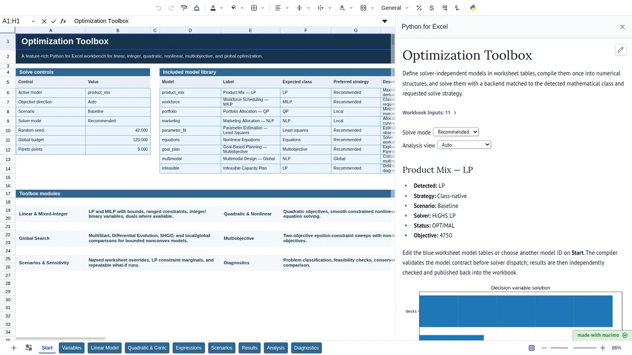
For a first run:
- Leave Start → Active model as
product_mixand Scenario asBaseline. - Review the blue decision-variable, objective, and constraint tables.
- Open Results and confirm
OPTIMALwith an objective of 4,750. - Switch Active model to
multimodalto compare local and bounded global methods. - Switch to
infeasibleto see how the workbench reports a model that cannot satisfy all constraints.
The Solve mode control selects a solve strategy independently of mathematical problem classification. Recommended uses the model catalog’s preferred strategy, Local requests one local solve, MultiStart repeats local solves from seeded starts, and Global requests the bounded global comparison for a continuous NLP with finite variable bounds and no general constraints.
For a guided tour, use Getting started.
Operating workflow
Author: an operations-research, finance, engineering, supply-chain, or quantitative analyst defines and validates the reusable model structure. The author owns variable semantics, objective direction, constraints, nonlinear expressions, solver assumptions, scenario definitions, scale choices, and acceptance tests.
Workbook user: a planner, analyst, reviewer, or manager changes approved worksheet inputs and scenarios, runs the workbook, and reviews decision values, binding constraints, feasibility evidence, tradeoffs, and solver diagnostics without needing to edit Python.
A typical recurring handoff is:
- The author creates or adapts a model using the documented worksheet schemas.
- The author validates the baseline and meaningful edge cases, including infeasibility where relevant.
- The workbook user changes business assumptions or selects a named scenario.
- The notebook recompiles and solves the same model.
- The workbook user reviews Results, Analysis, and Diagnostics before using the decisions downstream.
For recurring use, save the completed notebook and open it in App mode if that presentation is appropriate. App mode changes presentation; it does not change workbook permissions, hide source, or alter workbook trust.
Download the Excel template
Inputs and assumptions
Workbook map
| Sheet | Purpose | Primary user |
|---|---|---|
| Start | Active model, objective direction, scenario, solver mode, seed, global budget, Pareto density, and included-model catalog | Author and workbook user |
| Variables | Decision variables and scalar parameters | Author; selected values may be maintained by workbook user |
| Linear Model | Explicit objective definitions and senses, linear objective terms, ranged linear constraints, and sparse long-form coefficients | Author |
| Quadratic & Conic | Quadratic objective terms; conic support is explicitly planned, not active | Author |
| Expressions | Safe nonlinear objectives, nonlinear constraints, residuals, and equations | Author |
| Scenarios | Named overrides of parameters, variable bounds, objective coefficients, or constraint bounds | Author; workbook user selects scenario |
| Results | Normalized solve summary, decision variables, and constraint status | Workbook user/reviewer |
| Analysis | Pareto frontier, local/global solver comparison, LP marginals, or scenario availability depending on the active model | Workbook user/reviewer |
| Diagnostics | Classification evidence, feasibility checks, warnings, and solver limitations | Author and reviewer |
Important assumptions
- Model IDs are the join key. Every row belonging to a model uses the same
Modelvalue. - Variable and parameter names are machine-safe identifiers. Use letters, digits, and underscores; the first character must be a letter or underscore.
- Variable types are explicit. The beta accepts
Continuous,Integer, andBinary. Unsupported spellings fail validation instead of silently becoming continuous variables. - Blank bounds mean unbounded. A blank lower bound is negative infinity; a blank upper bound is positive infinity. Global search is stricter and requires finite bounds on every variable.
- Objective sense is part of the model. Each enabled objective is defined explicitly with
MinimizeorMaximize. Start → Objective direction defaults toAuto, which preserves that worksheet sense; an explicit Start override is allowed only for a single-objective model. - Scenario names are per model. Selecting a scenario applies only enabled rows for the active model and scenario name.
- Global budget is a browser-scale search budget, not a universal evaluation cap. Different algorithms consume it differently.
- Pareto analysis currently requires exactly two named linear objectives. It does not yet generalize to arbitrary nonlinear multiobjective problems.
The Modeling guide documents every input column and the supported expression language.
Notebook implementation
The workbook is backed by a notebook that performs four distinct jobs: ingestion, compilation, solving, and publication.
inputs = bf.inputs(
    controls=bf.ref("Start!A5:B12", headers=True),
    variables=bf.ref("Variables!A5:J40", headers=True),
    objectives=bf.ref("Linear Model!A5:F30", headers=True),
    linear_objectives=bf.ref("Linear Model!H5:L40", headers=True),
    constraint_defs=bf.ref("Linear Model!N5:T40", headers=True),
    constraint_terms=bf.ref("Linear Model!V5:Z80", headers=True),
    quadratic_terms=bf.ref("Quadratic & Conic!A5:F20", headers=True),
    expressions=bf.ref("Expressions!A5:I30", headers=True),
    scenarios=bf.ref("Scenarios!A5:G20", headers=True),
)
The notebook filters those ranges by active model, applies the selected scenario, validates identifiers and variable types, creates dense/sparse numerical representations as needed, and selects a solver path from the resulting mathematical structure.
The notebook then publishes one normalized contract regardless of solver family:
bf.publish(outputs={
    "summary": summary,
    "variables": variables_output,
    "constraints": constraints_output,
    "analysis": analysis,
    "diagnostics": diagnostics_rows,
})
That normalization is important for workbook handoff. A reviewer can use the same Results columns whether the underlying solve used HiGHS LP, HiGHS MILP, SLSQP, nonlinear least squares, a Pareto sweep, or a global-search comparison.
Safe nonlinear expressions
Worksheet nonlinear expressions are not passed to unrestricted Python. The notebook parses them with Python’s abstract syntax tree and accepts only arithmetic, known variable/parameter names, and these functions:
exp, log, sqrt, sin, cos, tanh, abs, minimum, maximum.
Supported operators are +, -, *, /, and **, including unary + and -. Attribute access, indexing, imports, comprehensions, keyword arguments, and arbitrary function calls are rejected.
See Modeling → Nonlinear expression language for the complete contract.
How the calculation/model works
1. Compile a model from worksheet rows
The compiler joins enabled rows on Model, validates names and bounds, applies scenario overrides, and constructs:
- the decision vector and variable bounds;
- integer/binary integrality flags;
- explicit objective metadata plus compiled linear, quadratic, and nonlinear objective components;
- a linear constraint matrix with independent lower and upper bounds;
- quadratic objective terms;
- compiled nonlinear expressions;
- nonlinear constraint functions;
- residual or equation vectors when applicable.
This is analogous in spirit to a problem-based modeling layer: the workbook describes the problem, while the compiler converts it into the numerical representation required by a solver.
2. Classify the narrowest supported problem family
Classification is structural and independent of solve strategy:
- Residual expressions → Least squares (currently bounds only).
- Equation expressions → Equations (currently bounds only).
- More than one enabled objective → Multiobjective, after validating the current two-linear-objective/continuous-variable contract.
- Any integer/binary variable → MILP, provided the model is linear.
- Nonlinear objective or nonlinear constraint → NLP.
- Quadratic objective terms → QP.
- Otherwise → LP.
The compiler rejects unsupported combinations before solver dispatch rather than silently dropping model structure. The classifier does not infer convexity; in particular, a user-authored quadratic objective is not automatically certified convex. Global is a solve strategy for a bounded NLP, not a problem class.
3. Dispatch to a solver family
| Detected class | Default beta path | Result claim |
|---|---|---|
| LP | HiGHS through scipy.optimize.linprog |
OPTIMAL, INFEASIBLE, UNBOUNDED, or FAILED from the mathematical-programming solver status |
| MILP | HiGHS through scipy.optimize.milp |
Same conservative discrete status mapping |
| QP | SLSQP through scipy.optimize.minimize |
Local constrained solution; LOCAL_OPTIMUM when successful and independently feasible |
| NLP | SLSQP; optional bounded global comparison | Local or BEST_FOUND depending on mode |
| Least squares | scipy.optimize.least_squares |
LOCAL_OPTIMUM when the residual solve succeeds |
| Equations | least_squares on equation residuals |
FEASIBLE_SOLUTION only when residual norm is within tolerance |
| Multiobjective | Repeated HiGHS LP solves with an epsilon constraint | PARETO_SET for the returned tradeoff table |
| NLP + Global strategy | Local + MultiStart + Differential Evolution + SHGO | BEST_FOUND; no unsupported global-optimum certification |
The Solver guide explains when those mappings are appropriate and where they differ from MATLAB.
4. Check feasibility independently
Solver success alone is not accepted as the workbook’s final evidence. The notebook recomputes violation against:
- variable lower and upper bounds;
- integer/binary integrality;
- linear constraint lower and upper bounds;
- supported nonlinear constraint lower and upper bounds.
The maximum modeled violation is published in the summary. A nominally successful local or global solve is downgraded to FAILED if violation exceeds 1e-6.
5. Normalize results for Excel
The same five publications feed the workbook:
- summary — model, class, scenario, solver, status, objective, maximum violation, runtime, evaluation/node count, seed, and a concise termination message;
- variables — decision value, bounds, bound status, and solver marginal where implemented;
- constraints — activity, bounds, slack, binding flag, and LP marginal where available;
- analysis — Pareto points, solver comparison, current solve plus scenario availability, or LP marginal rows;
- diagnostics — structural, numerical, feasibility, runtime, and capability notes.
For solver-specific formulation details, status semantics, and algorithm limitations, use the Solver guide. For MultiStart, Differential Evolution, SHGO, reproducibility, and claim strength, use Global optimization. The overview intentionally stops at the stable compiler/result contract so implementation detail has one authoritative home.
Validation / expected results
The Toolbox is validated at several layers because a solver result can be numerically plausible while the workbook integration is wrong.
| Fixture | Model ID | Family | Expected evidence |
|---|---|---|---|
| Product Mix | product_mix |
LP | OPTIMAL; objective 4,750; zero independent violation; LP marginal rows available |
| Workforce Scheduling | workforce |
MILP | OPTIMAL; integer shift-start decisions; staffing constraints satisfied |
| Portfolio Allocation | portfolio |
QP | LOCAL_OPTIMUM; risk ≈ 0.01212943; weights ≈ 0.418607 / 0.352154 / 0.229239; return constraint binds at 0.07 |
| Marketing Allocation | marketing |
NLP | LOCAL_OPTIMUM; budget-constrained nonlinear response allocation |
| Parameter Estimation | parameter_fit |
Least squares | LOCAL_OPTIMUM; bounded fitted parameters and reduced residual sum of squares |
| Nonlinear Equations | equations |
Equations | FEASIBLE_SOLUTION; small equation residual norm |
| Goal-Based Planning | goal_plan |
Multiobjective | PARETO_SET; nondominated cost/emissions tradeoff rows |
| Multimodal Design | multimodal |
NLP + Global strategy | BEST_FOUND; local/global methods compared without a false proof-of-globality claim |
| Infeasible Capacity Plan | infeasible |
LP diagnostics | INFEASIBLE; no fabricated decision vector |
The canonical template gate also checks:
- reproducible generation of
workbook.xlsxandworkbook.jsonfromworkbook.py; - that the notebook embedded in the XLSX exactly matches
notebook.py; - that every
BF.OUTPUTpublication matches the finished workbook contract; - strict notebook structure;
- native execution of every baseline/scenario vector in
offline_test.py; - real browser/Pyodide execution through the offline workbook host;
- generated walkthrough-poster readiness;
- worksheet edit/restore behavior in the Univer integration;
- runtime output presentation and semantic formatting checks.
For production use, the author should add domain-specific acceptance cases beyond the included generic fixtures.
Limitations
The beta deliberately documents unsupported areas rather than presenting the MATLAB inspiration as parity.
Modeling limits
- New objectives require an explicit
Sense; Objective direction = Auto preserves that worksheet definition. - The current multiobjective engine requires exactly two named linear objectives.
- The quadratic compiler does not certify convexity.
- The safe expression language is intentionally smaller than Python or MATLAB.
- The authored input bands are finite worksheet ranges; large operational models should be designed and benchmarked rather than pasted blindly into the fixture layout.
Solver limits
- QP uses general SLSQP rather than a dedicated QP backend.
- There is no active SOCP backend.
- There is no semi-infinite optimization.
- There is no automatic differentiation.
- There is no dedicated derivative-free local pattern-search implementation in the current release.
- Genetic algorithms, particle swarm, simulated annealing, and surrogate optimization are not currently implemented.
- Browser Python is single-worker for this application; there is no MATLAB-style parallel MultiStart/global-search mode.
- Global methods require finite variable bounds in the current workbench.
- Global methods report
BEST_FOUND; the beta does not certify mathematical global optimality from stochastic search.
Sensitivity limits
- LP constraint marginals are local shadow-price information from the current optimal solution.
- Full objective/RHS allowable-increase/decrease ranging is not yet exposed.
- MILP, nonlinear, and global sensitivity should be evaluated by explicit scenario perturbations rather than treating LP dual concepts as transferable.
Operational limits
- Browser-scale evaluation budgets are intentionally conservative.
- Solver runtime depends strongly on dimension, conditioning, integrality, and nonlinear evaluation cost; the included small fixtures are not model-size benchmarks.
- The workbook is a modeling and review surface, not a remote optimization server or long-running batch system.
When to use this approach
Use this Toolbox when the optimization model itself belongs in the workbook handoff. It is particularly well suited when:
- business users need to inspect assumptions and constraints in Excel;
- an analyst wants several solver families behind one auditable schema;
- scenarios should be reusable worksheet records rather than workbook copies;
- reviewers need explicit feasibility/slack/status evidence;
- local-versus-global behavior is part of the decision discussion;
- a Pareto frontier is more useful than collapsing competing objectives into one opaque score;
- the model is small or medium enough for interactive browser execution.
Prefer a dedicated Python service or optimization platform when models require very large sparse instances, long-running distributed search, specialized commercial solvers, high-throughput batch solving, or solver features that the current capability map marks unavailable.
How this compares with MATLAB and Excel
The workbench is intended for a specific middle ground: optimization is substantial enough to deserve a reusable model/compiler/result contract, but the assumptions and outputs still need to remain visible and operable in Excel.
| Starting point | Best fit | Main tradeoff |
|---|---|---|
| Native Excel | Goal Seek, Data Tables, Scenario Manager, formulas, and small transparent what-if models | No general reusable constrained-optimization engine |
| Microsoft Solver Add-in | A relatively small optimization already expressed naturally as worksheet formulas | Dialog/cell-address workflow is less suited to a generic multi-family model contract |
| Python for Excel Optimization Toolbox | Reusable table-defined LP/MILP/QP/NLP/fitting/equation/Pareto workflows with normalized diagnostics and workbook handoff | Browser-scale limits; fewer specialized algorithms than a numerical-computing product |
| MATLAB Optimization + Global Optimization Toolboxes | Broad specialist numerical optimization, dedicated algorithms, advanced derivatives, conic/global methods, larger scientific workflows | MATLAB-centric environment rather than an Excel-first application surface |
This is a capability comparison, not API compatibility. The Toolbox borrows a useful optimization problem taxonomy, but it does not implement MATLAB function signatures and does not attempt to replace ordinary Excel formulas or Solver for simple worksheet-native cases.
For detailed solver-by-solver comparison with MATLAB Optimization Toolbox, see Solvers → MATLAB capability comparison. For MATLAB Global Optimization Toolbox, see Global optimization → Comparison with MATLAB Global Optimization Toolbox.
Which one should you use?
| Situation | Best starting point |
|---|---|
| One target formula and one unknown input | Excel Goal Seek |
| One-/two-variable sensitivity grid | Excel Data Table |
| Small constrained model already expressed as worksheet formulas | Microsoft Solver Add-in |
| Reusable Excel optimization with structured scenarios, standardized outputs, diagnostics, or several problem families | Python for Excel Optimization Toolbox |
| Compare local, MultiStart, and bounded global search inside the workbook handoff | Python for Excel Optimization Toolbox |
| Dedicated QP/conic algorithms, automatic differentiation, specialized global algorithms, parallel optimization, or MATLAB-centric engineering/scientific workflows | MATLAB Optimization / Global Optimization Toolboxes |
| Very large, long-running, distributed, or commercial-solver workloads | A dedicated optimization service/platform |
External capability references are maintained in the solver/global guides rather than duplicated here.